Introduction to Data Modelling
Think of data modeling as the architectural blueprint for a database. Before pouring the concrete or writing a single line of SQL, data models provide a clear visual representation of the major data subjects, their underlying attributes, how they interact with one another, and the strict business rules that govern them. It ensures that the database will be built to accurately reflect the business’s actual needs.
To navigate this process, you need to understand three core building blocks:
- Entity: A real-world object, concept, or event that needs to be tracked within the database. Examples include a
Customer, aProduct, or aSales Transaction. - Attributes: The specific characteristics, properties, or traits that describe an entity. For a
Customerentity, the attributes might includeCustomer_Name,Age,Email_Address, andRegistration_Date. - Relationship: The logical association or interaction between two or more entities. For example, a
Customerplaces anOrder. This relationship dictates how tables will eventually connect to one another.
The Three Phases of Data Modeling
Designing a database is an iterative process. Data modeling is typically broken down into three distinct phases, moving from high-level business concepts to deeply technical database schemas:
- Conceptual Data Model: This is the 30,000-foot view. It describes what the system contains by mapping out the core business entities and their basic relationships. It deliberately ignores technical implementation details, making it the perfect tool for communicating with business stakeholders and aligning on the overarching data requirements.
- Logical Data Model: This phase dives deeper into the how, but remains independent of any specific Database Management System (DBMS). It adds flesh to the conceptual model by fully defining all attributes, setting data constraints, establishing primary and foreign keys, and finalizing the exact logical relationships between entities.
- Physical Data Model: This is the final, highly technical blueprint that describes exactly how the system will be implemented using a specific technology (e.g., PostgreSQL, Snowflake, or Oracle). It defines the physical storage structures, exact data types (like
VARCHARorINT), indexing strategies for performance, partitioning, and access methods.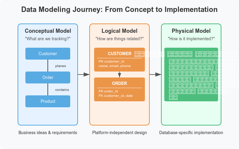
Cardinality and Crow’s Foot Notation
When defining relationships between entities, we must establish the cardinality, which refers to the numerical nature of the relationship (often expressed by mapping the minimum and maximum occurrences).
The three primary types of cardinality are:
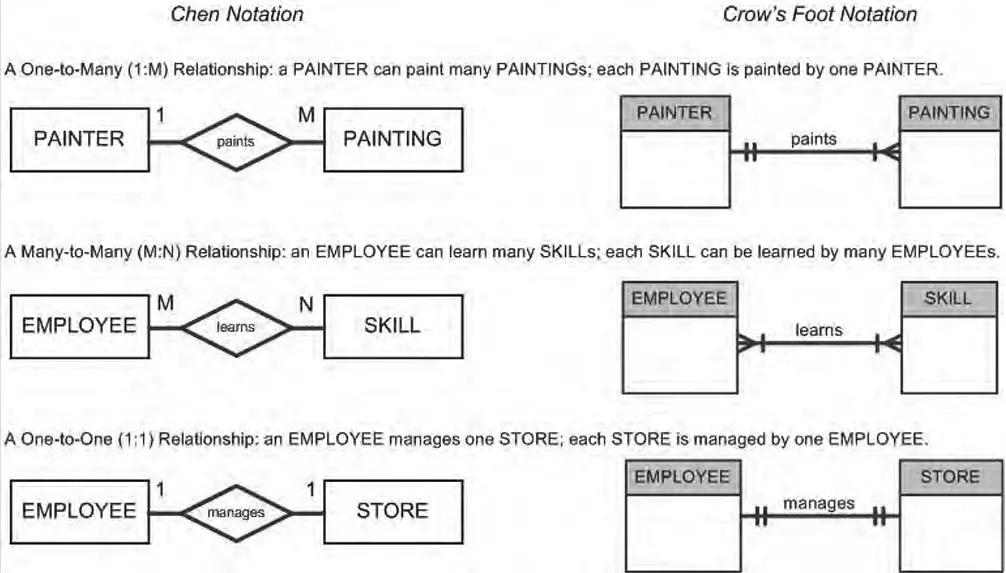
- One-to-One (1:1): Each instance of Entity A is related to exactly one instance of Entity B, and vice versa. (e.g., One
Employeehas exactly oneID Badge). - One-to-Many (1:N): One instance of Entity A can be related to many instances of Entity B, but an instance of Entity B relates to only one instance of Entity A. (e.g., One
Customercan place manyOrders, but anOrderbelongs to only oneCustomer). - Many-to-Many (M:N): Instances in Entity A can relate to multiple instances in Entity B, and vice versa. (e.g.,
Studentsenrolling in multipleClasses). In relational databases, this is typically resolved by creating a junction/mapping table between them.
Crow’s Foot Notation is the industry-standard visual language used in Entity-Relationship Diagrams (ERDs). It uses specific symbols—such as straight lines, open circles (optionality), and branching “crow’s feet” (multiple)—to clearly illustrate these complex cardinality constraints at a glance.
Normalization vs. Denormalization
Two opposing forces dictate how data is structured, depending entirely on the system’s end goal (OLTP vs. OLAP).
Normalization
Normalization is a rigorous process of organizing data to reduce redundancy and improve data integrity. It involves breaking down large, complex tables into smaller, highly structured tables linked by relationships. By following strict mathematical rules known as Normal Forms (such as 1NF, 2NF, and 3NF), normalization eliminates data anomalies during insertion, updating, or deletion.
- Use Case: It is the gold standard for transactional databases (OLTP) where preventing data duplication and ensuring absolute accuracy are top priorities.
Denormalization
Denormalization is the strategic reverse of normalization. It involves intentionally combining multiple tables and reintroducing redundant data into a single, massive table. While this violates normalization rules and risks data duplication, it drastically reduces the need for computationally expensive JOIN operations.
- Use Case: This is highly favored in data warehousing and analytical systems (OLAP), where the primary goal is to maximize read performance and query speed over massive volumes of historical data.

Dimensional Modelling
Pioneered by Ralph Kimball, dimensional modeling is a specialized database design technique used extensively in building enterprise Data Warehouses and Data Marts. Instead of aiming for perfect normalization, it organizes data into a structure that is highly intuitive for business users and optimized for fast analytical querying.
It revolves around two foundational concepts:
- Fact Tables: The core measurements, metrics, or quantitative data of a business process (e.g.,
Sales_Amount,Discount,Quantity_Sold). Facts are usually massive, narrow tables containing numbers and keys. - Dimension Tables: The context surrounding the facts. Dimensions answer the who, what, where, when, and why. (e.g.,
Customer_Demographics,Store_Location,Date_Calendar). They are typically wide tables filled with descriptive text used to filter and group data.
Schemas in Dimensional Modeling
- Star Schema: The simplest and most widely used design. A single, massive Fact table sits in the center, directly connected to multiple denormalized Dimension tables, resembling a star. It offers incredibly fast read performance.
- Snowflake Schema: A variation where the Dimension tables are normalized into multiple related tables. It saves storage space but requires more complex joins, looking visually like a snowflake.
Keys and Historical Tracking
To ensure rock-solid data integrity within these models, engineers rely on specific keys:
- Surrogate Keys: Artificial, system-generated integer keys (e.g.,
1, 2, 3...) used as primary keys in dimension tables, shielding the warehouse from changes in the operational source systems. - Natural Keys: The original operational ID from the source system (e.g.,
Invoice_Number_ABC123). - Foreign Keys: Used in the Fact table to map back to the primary surrogate keys in the Dimension tables.
Finally, managing how attributes change over time is handled by Slowly Changing Dimensions (SCD) policies:
- Type 1 (Overwrite): Updates the old data with new data. History is lost.
- Type 2 (Unlimited History): Adds a new row for every change, tracking the full historical timeline (often using effective dates).
- Type 3 (Limited History): Adds a new column to track only the current and previous value.
